SapBERT

• 创建日期：2026-05-14

Self-Alignment Pretraining for Biomedical Entity Representations

To learn:

• t-SNE
• download some data from UMLS and look what they like, how to use
• ADAPTER module: a fine-tune module, we could directly learn LoRA/DoRA/RAG, the popular fine tune skill
• MS loss， different loss function

1. To understand list

• Entity linking ✅
• medical entity linking ✅
• metric ✅
• self-align ✅

2. Abstract

• SapBERT is a pretraining model that self-aligns the representation space of biomedical entites
• Solves problem that accurately capturing fine-grained semantic relationships in the biomedical domain remains a challenge.
• Solves problem by design a scalable metric learning framework that can leverage UMLS
• Achieve a new SOTA on six MEL benchmarking datasets.

3. Related works:

4. Introduction:

• Problem1: The heterogeneous naming of biomedical concepts poses a major challenge to representation learning.
• Solution1: MEL addresses problem1 by framing it as a task of mapping entity mentions to unified concepts in a medical knowledge graph.
• Problem2 of the solution1: The main bottleneck of MEL is the quality of the entity representations
• Solution2a: Adopts very sophisticated text pre-processing heuristics
• Solution2b: Uses self-supervised-learning
• Problem3 of solution2a and 2b: Representing medical entities with the existing SOTA pretrained MLMs does not lead to a well-separated representation space.
• Solution3 (proposed solution): Pretrains a Transformer-based language model on UMLS and designs a self-alignment objective that clusters synonyms of the same concept, and samples hard training pairs from the knowledge base and use a scalable metric learning loss.

To understand of introduction:

• t-SNE
• understand what actually the data like in UMLS
• ADAPTER module
• self-alignment objective

5. Methods:


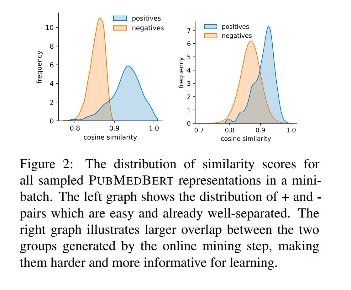
What's the meaning of figure2, what does the author want to imply?

To understand of methods:

• metric learning framework ✅
• what is online hard pairs mining ??? ✅
• what does "violate the following condition" mean, satisfied or unsatisfied?? ✅
• Formula(2): MS loss ✅
• Why MS loss performs better than other loss function, how to understand?? Table 6 ✅

Question of formula(2):

• There are many positive samples, do we compute each positive sample with each negative sample?? ✅

6. Experiments:

To understand of experiments:

• tradenames ✅
• How to ensure sufficient positives present in each mini-batch(Blue highlighted in Data preparation details) ✅
• How to fine-tune, why we might need to fine-tune our model ✅
• What is "BERT + SapBERT", how to plus SapBERT based on BERT?? ✅
• "Impact of online mining": If we switch off online hard mining, how could we find the negative samples and train the model ✅

I skip the "The ADAPTER Variant" part

Actual compute steps of online hard samples mining

第一步：计算全成对相似度矩阵 $S$

首先，将 Mini-batch 中 $b$ 个实体的特征向量（由 BERT 输出的 [CLS] 向量 ）表示为矩阵 $F \in \mathbb{R}^{b \times d}$。

1. 计算矩阵 $S$：通过 $S = F \cdot F^T$（假设向量已归一化）得到一个 $b \times b$ 的相似度矩阵 。
2. 矩阵含义：$S_{ij}$ 代表第 $i$ 个实体和第 $j$ 个实体之间的余弦相似度 。

第二步：构建标签掩码 (Label Masks)

为了区分哪些是“自己人”（同义词），我们需要利用标签（CUI）：

1. 正样本掩码 ($M_{pos}$)：如果第 $i$ 个实体和第 $j$ 个实体的 CUI 相同，则 $M_{pos}[i, j] = 1$，否则为 0 。
2. 负样本掩码 ($M_{neg}$)：如果 CUI 不同，则 $M_{neg}[i, j] = 1$，否则为 0 。
3. 注意：通常会排除对角线（即自己和自己）。

第三步：利用 $S$ 进行在线硬采样

虽然论文公式使用的是欧几里得距离 $||\cdot||_2$ ，但在单位向量下，距离和余弦相似度是可以互换的：$||u-v||_2^2 = 2 - 2 \cdot \cos(u, v)$。 实际的筛选逻辑如下：

1. 转换条件：将距离公式转化为相似度公式。违反距离条件等同于： $S_{ap} < S_{an} + \text{margin}$ （这里的 $\text{margin}$ 对应论文中的 $\lambda$，通常取小负数，如 -0.2 ）。
2. 批量寻找硬三元组：
   • 对于每一个锚点 $i$：
   • 从 $S[i, :]$ 中通过 $M_{pos}$ 找出所有的正样本相似度 $\{S_{ip}\}$。
   • 从 $S[i, :]$ 中通过 $M_{neg}$ 找出所有的负样本相似度 $\{S_{in}\}$。
   • 判定硬样本：如果某对 $(p, n)$ 满足 $S_{ip} - S_{in} < \text{margin}$，则记录索引 $p$ 为硬正样本，索引 $n$ 为硬负样本 。

第四步：计算 MS Loss (公式 2 的具体实现)

现在你拥有了每个锚点 $i$ 对应的硬正样本集 $\mathcal{P}_i$ 和硬负样本集 $\mathcal{N}_i$ 。接下来带入公式 (2) 进行求和 ：

1. 处理负样本项（Push）：
   • 计算 $\sum_{n \in \mathcal{N}_i} e^{\alpha(S_{in} - \epsilon)}$。
   • 这会给那些相似度极高（错误地很像锚点）的负样本极大的权重 。
2. 处理正样本项（Pull）：
   • 计算 $\sum_{p \in \mathcal{P}_i} e^{-\beta(S_{ip} - \epsilon)}$。
   • 这会给那些相似度极低（离锚点太远）的正样本极大的权重 。
3. 对数求和：对上述两项取 $\log(1 + \dots)$ 并乘以温度系数 $1/\alpha$ 或 $1/\beta$ 。
4. 最终平均：对批次内所有锚点产生的损失求平均，得到最终 $\mathcal{L}$ 。 MS Loss 的数学表达式如下 ： $\mathcal{L}=\frac{1}{|R_{0}|}\sum_{i=0}^{|R_{0}|} \left( \underbrace{\frac{1}{\alpha}\log(1+\sum_{n\in\mathcal{N}_{i}}e^{\alpha(S_{in}-\epsilon)})}_{\text{负样本项 (Push)}} + \underbrace{\frac{1}{\beta}\log(1+\sum_{p\in\mathcal{P}_{i}}e^{-\beta(S_{ip}-\epsilon)})}_{\text{正样本项 (Pull)}} \right)$